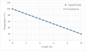
How to Analytically Solve the Cylindrical Heat Equation

In the previous post we looked at the analytical solution to the Cartesian heat conduction equation. This equation cannot predict the temperature drop through cylindrical systems such as pipes so in this post we will look at the analytical solution for the cylindrical heat equation. We will look at the simplest form of this which is for steady, one-dimensional heat transfer.

Steady, One-Dimensional Cylindrical Heat Equation

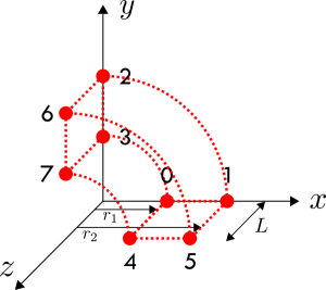
The cylindrical heat equation has been shown in Eq. 1 (this was discussed here) for a constant thermal conductivity solid. The steady solution implies that the time derivative will cancel from Eq. 1. We need to be a little careful with the treatment of the remaining three terms which represent heat transfer in each direction. Each term looks a little bit different – unlike the Cartesian system where each term looked the same and only varied in whether there was an $x$ , $y$ or $z$ present. One-dimensional heat transfer implies we can only have one of these derivatives present, but which one depends on the case we consider. To help clarify this, look at Figure 1 below.

Cylindrical heat transfer — Figure 1. Directions of heat transfer for a cylindrical system.

If we are considering radial heat transfer, then we should leave the $r$ term. If we consider axial heat transfer, then we should leave the $z$ term (in this case the solution will be the same as the Cartesian system). And if we consider circumferential (sometimes called azimuthal) heat transfer then we should leave the $\phi$ term.

Each of these cases is valid, however here we consider the radial case as this can be best replicated in pipe flow systems which have fluid streams on both sides of the pipe. If the fluids are held at different temperatures, there will be radial temperature variations present. This is actually quite common – hot water in pipes, steam in a boiler, condensing vapour in a refrigerator. Based on this simplification, we arrive at Eq. 2 for the heat equation. It becomes an ordinary differential equation (ODE) since temperature is a function of the radial direction only.

\frac{1}{r}\frac {\partial}{\partial r}\left(r\frac{\partial T}{\partial r}\right)+\frac{1}{r^2}\frac {\partial}{\partial \phi}\left(\frac{\partial T}{\partial \phi}\right)+\frac {\partial}{\partial z}\left(\frac{\partial T}{\partial z}\right) = \frac{1}{\alpha}\frac {\partial T}{\partial t} \tag*{Eq. 1}

\frac{1}{r}\frac {d}{d r}\left(r\frac{d T}{d r}\right)=0

\frac {d}{d r}\left(r\frac{d T}{d r}\right)=0 \tag*{Eq. 2}

Note that we can drop the $1/r$ term since this cannot equal zero for any reasonable $r$ value and thus the derivative must. This ODE is slightly more complicated to solve than the Cartesian counterpart. Still, we can integrate this twice to obtain the general solution.

\int\frac {d}{d r}\left(r\frac{d T}{d r}\right)dr=\int0dr

r\frac{d T}{d r}=A

\frac{d T}{d r}=\frac{A}{r}

\int\frac{d T}{d r}dr=\int\frac{A}{r}dr

T=A\ln(r)+B \tag*{Eq. 3}

Thus the general solution in Eq. 3 is $T=A\ln(r)+B$ . $A$ and $B$ are constants which, like the Cartesian system, depend on the boundary conditions and require us to evaluate them. Note that we have a logarithmic solution, rather than the straight line solution for the Cartesian system. This arises purely due to the radial system under consideration and the fact that we need to integrate a $1/r$ term.

There are many logarithmic lines which satisfy our ODE, any combination of $A$ and $B$ will do. We need to know these values specifically for our case and this is easiest done for fixed temperature boundary conditions. Two of these are required to completely specify the problem, one at each boundary. These have been shown below. BC 1 states that the temperature at $r=r_1$ i.e. the inside of the pipe is equal to $T_1$ and BC 2 states that the temperature at $r=r_2$ i.e. the outside of the pipe is equal to $T_2$ . Such a system has been shown in Figure 2.

T(r=r_1)=T_1\tag*{BC 1}

T(r=r_2)=T_2\tag*{BC 2}

These boundary conditions can be substituted into Eq. 3 to find values of $A$ and $B$ . We have two equations with two unknowns which can be solved simultaneously. This leads to values for $A$ and $B$ as shown in Eq. 4 and Eq. 5. The particular solution to the heat equation in cylindrical coordinates is shown in Eq. 6. We need to make use of some log laws in this such as the quotient log law i.e. $\ln(a/b)=\ln(a)-\ln(b)$ . Note that the exact method followed in this procedure may alter the form obtained and as a result you may see this presented differently in various sources.

A=\frac{T_1-T_2}{\ln(r_1/r_2)}\tag*{Eq. 4}

B=T_1-\frac{T_1-T_2}{\ln(r_1/r_2)}\ln(r_1)\tag*{Eq. 5}

T=\frac{T_1-T_2}{\ln(r_1/r_2)}\ln\left(\frac{r}{r_1}\right)+T_1\tag*{Eq. 6}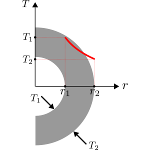

Cylindrical one dimensional heat transfer solution — Figure 2. The temperature distribution in a radial system.

This is the solution to the heat equation for a radial system (a simplified cylindrical system). With it we can plot the temperature distribution in a pipe wall when the inner and outer temperatures are held constant. This has been shown in Figure 2 to the side.

Being able to plot the temperature distribution lets us know the rate of heat transfer through the pipe wall which is very useful for many applications. The last system we will look at before moving onto more complex boundary conditions is the spherical system. This is actually much less common in practice, but is still useful to be able to derive the analytical temperature distribution for this.