Heat Conduction Equation with Mixed Boundary Conditions

In some of the previous posts, we looked at solutions to the heat conduction equation in Cartesian coordinates with temperature, flux and convective boundary conditions for both boundaries of a steady, one-dimensional system. We can actually mix and match these boundaries so in this post we will go over some possible combinations and look at the solutions for these.

Temperature and convection

Temperature and convective boundary conditions for heat conduction equation — Figure 1. The one-dimensional system with a temperature and convection boundary condition.

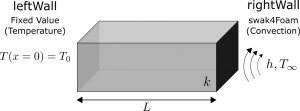
We could consider the system as shown in Figure 1 which combines the temperature and convection boundary conditions into a single system. The left boundary is kept at a fixed temperature of $T_0$ and the right boundary is subject to convection within a fluid with heat transfer coefficient of $h$ and ambient temperature of $T_{\infty}$ .

The boundary conditions for this case are shown in BC 1 and BC 2.

T(x=0)=T_0\tag*{BC 1}

\left. -k \frac{dT}{dx} \right|_{x=L}=h(T_L-T_{\infty})\tag*{BC 2}

These can be substituted into the general solution to the heat equation for a steady, one-dimensional Cartesian system $T=Ax+B$ to find the unknown constants $A$ and $B$ . One key point to remember is that we want to find the solution independent of $T_L$ as this typically isn’t available in these scenarios but the ambient temperature $T_\infty$ is.

BC 1 can be used first to find the value for $B$ by substitution into $T=Ax+B$ . From this we find that $B=T_0$ . Using this, we can then substitute this into BC 2, along with the fact that $dT/dx=A$ to yield the expression $-kA=h(AL+T_0-T_\infty)$ . By re-arranging this expression we end up with a expression for $A = (h(T_\infty -T_0))/(hL+k)$ . We can now find the solution for the temperature distribution to be as per Eq. 1.

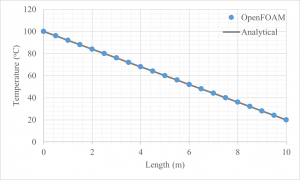
T=\frac{h(T_\infty -T_0)}{hL+k}x+T_0 \tag*{Eq. 1}

This is the solution we require. The temperature distribution can now be plotted as a function of $x$ for the case with one fixed temperature and one convective boundary.

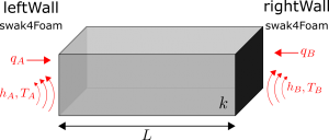
Note that we could have arrived at the same equation for temperature distribution had we used the expression developed in this post and assumed that $h_A$ was equal to infinity. This is to say that the temperature boundary condition is a special case of the convection boundary condition with the heat transfer coefficient set to infinity.

Flux and temperature

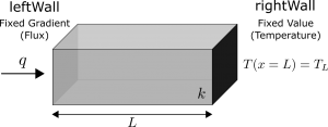
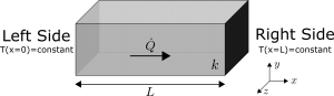
We could consider the system as shown in Figure 2 which combines the flux and temperature boundary conditions into a single system. The left boundary is subject to a constant heat flux $q$ and the right boundary is subject to a constant temperature $T_L$ .

The boundary conditions for this case are shown in BC 3 and BC 4.

These can be substituted into the general solution to the heat equation for a steady, one-dimensional Cartesian system $T=Ax+B$ to find the unknown constants $A$ and $B$ .

q=\left. -k \frac{dT}{dx} \right|_{x=0}\tag*{BC 3}

T(x=L)=T_L\tag*{BC 4}

We first recognise that the derivative of the general solution is $dT/dx = A$ which implies using BC 3 that $A = -q/k$ . Next we use BC 4 to find $B$ by evaluating the general solution at $x=L$ and setting this equal to $T_L$ as per BC 4. Solving for $B$ yields $B=T_L+qL/k$ . We can now find the solution for the temperature distribution to be as per Eq. 2.

T=\frac{q}{k}(L-x)+T_L \tag*{Eq. 2}

This is the solution we require. The temperature distribution can now be plotted as a function of $x$ for the case with one flux boundary and one fixed temperature boundary.

The process for finding the temperature distribution should be familiar at this point for the steady, one-dimensional Cartesian system with either temperature, flux or convective boundary conditions. The general solution is always $T=Ax+B$ and we just need to use the two boundary conditions to find the values of $A$ and $B$ .

In the case of the temperature boundary condition, the formulation is quite simple since we know the value at the boundary and will have an equation like $T(x=0/L) = T_{0/L}$ . In the case of the flux or convection boundary condition, the formulation is a bit more complicated as it relates to the derivative at the boundary and is based on an energy balance at the boundary. We will look at an even more complicated boundary condition in the next post which combines both the flux and convection boundary conditions into one boundary.

Note that the solution to the heat equation in each of these cases is dependent on boundary conditions. Unfortunately, if the boundary conditions were reversed in either of the case i.e. convection on the left and temperature on the right in the first case, or flux on the right and temperature on the left in the second case, then we would need to derive a new equation for the temperature distribution since the boundary conditions have changed.