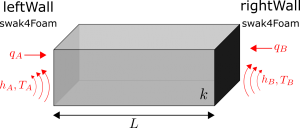
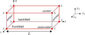
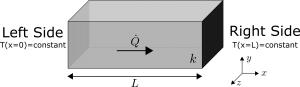
Heat Conduction Equation with Combined Boundary Conditions

In this post we are going to look at a more general boundary which combines multiple types of boundary conditions together. This is a nice exercise in solving an ordinary differential equation with quite complicated boundary conditions and it also produces a temperature distribution which can be used for a wide range of scenarios. As has been the case for these posts, we will look at the steady, one-dimensional Cartesian system as shown in Figure 1.

Mixed boundary conditions for heat conduction equation — Figure 1. The steady, one-dimensional Cartesian system with combined boundary conditions.

This system has both flux and convective boundaries on the left and right sides. On the left hand boundary we have heat flux $q_0$ entering and convection via a fluid with free-stream temperature of $T_A$ and heat transfer coefficient of $h_A$ . On the right hand boundary we have heat flux $q_L$ leaving and convection via a fluid with free-stream temperature of $T_B$ and heat transfer coefficient of $h_B$ .

The key to develop expressions for each boundary condition is to consider conservation of energy applied to the boundary. Since the boundary itself cannot store any energy as it has no volume associated with it, the energy entering the boundary must be equal to the energy leaving the boundary. For the left hand boundary, the energy transferred via flux and convection must equal the energy transferred via conduction within the solid. The same can be said of the right hand boundary. This has also been schematically shown in Figure 1. These boundary conditions can thus be represented in BC 1 and BC 2 for the left and right boundaries, respectively.

q_0+h_A(T_A-T_0)=-k\left. \frac{dT}{dx}\right |_{x=0} \tag*{BC 1}

q_L+h_B(T_L-T_B)=-k\left. \frac{dT}{dx}\right |_{x=L} \tag*{BC 2}

The general solution to the steady, one-dimensional heat equation has been shown in Eq. 1 with $A$ and $B$ constants that need to be determined from the boundary conditions above.

T=Ax+B \tag*{Eq. 1}

From the general solution in Eq. 1 we can deduce that the temperature gradient must be equal to a constant as shown in Eq. 2.

\frac{dT}{dx}=A\tag*{Eq. 2}

The process for finding $A$ and $B$ is a bit complicated due to the boundary conditions. It is best to express the temperature at the left ( $T_0$ ) and right ( $T_L$ ) wall as in Eq. 3 and Eq. 4, respectively. This makes the system simpler to solve and will also yield a result which is independent of wall temperatures $T_0$ and $T_L$ since these are normally unknown in the analysis.

T_0:T(x=0)=A\cdot 0+B=B\tag*{Eq. 3}

T_L:T(x=L)=A\cdot L+B=AL+B\tag*{Eq. 4}

We can substitute Eq. 3 and Eq. 4 into BC 1 and BC 2 to yield new expressions for the boundary conditions.

q_0+h_A(T_A-B)=-kA \tag*{BC 1A}

q_L+h_B(AL-B-T_B)=-kA \tag*{BC 2A}

We now have two equations with two unknowns ( $A$ and $B$ ) that can be solved simultaneously. This is a bit of a tedious process, but here we rearranged BC 1A in terms of $B$ (i.e. $B=1/h_A(q_0+h_A T_A+kA)$ ) and then substituted this into BC 2A. After doing this we can simplify the resulting expression and obtain a value for $A$ . We get the following.

A=\frac{h_Ah_B\left[ (T_B-T_A)-\frac{q_0}{h_A}-\frac{q_L}{h_B}\right]}{h_Ah_BL+k(h_A+h_B)} \tag*{Eq. 5}

And then the expression for $B$ can be found from the rearranged BC 1A as:

B=T_A+\frac{q_0}{h_A}+\frac{k}{h_A}\frac{h_Ah_B\left[ (T_B-T_A)-\frac{q_0}{h_A}-\frac{q_L}{h_B}\right]}{h_Ah_BL+k(h_A+h_B)} \tag*{Eq. 6}

These two constants can be placed into the general solution of Eq. 1 to yield the solution for the case with combined boundary conditions on both boundaries. This lengthy expression is given in Eq. 7.

T=Ax+B

T=\frac{h_Ah_B\left[ (T_B-T_A)-\cfrac{q_0}{h_A}-\cfrac{q_L}{h_B}\right]}{h_Ah_BL+k(h_A+h_B)}x+T_A+\cfrac{q_0}{h_A}+\frac{k}{h_A}\cfrac{h_Ah_B\left[ (T_B-T_A)-\cfrac{q_0}{h_A}-\cfrac{q_L}{h_B}\right]}{h_Ah_BL+k(h_A+h_B)}

T=T_A+\cfrac{q_0}{h_A}+\frac{h_Ah_B\left[ (T_B-T_A)-\left(\cfrac{q_0}{h_A}+\cfrac{q_L}{h_B}\right)\right]}{h_Ah_BL+k(h_A+h_B)}\left(x+\frac{k}{h_A}\right) \tag*{Eq. 7}

Although this equation doesn’t look particularly nice, it does tell us quite a lot about many different systems. Because we used combined boundary conditions we can use it for several cases just by setting appropriate values:

Cases involving only convection on both sides can be modelled by setting $q_0$ and $q_L$ to zero.
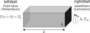
Cases involving temperature on both sides can be modelled by setting $q_0$ and $q_L$ to zero and $h_A$ and $h_B$ to very large values.
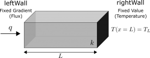
A case involving only flux on both sides can be modelled by setting $h_A$ and $h_B$ to small values (be careful with this one, you can get some strange results!).
And basically everything else in between.

Practically, we might want to use this equation for a system which has both flux and convection present on one or both of the surfaces. Imagine sunlight striking the surface of the earth or an outside facing wall which also has wind blowing over it. The sunlight could be modelled as a flux boundary condition and the environment could be modelled as a convection boundary condition. A screen which is emitting light often has fluid passing over it as well which this equation could suit.

Also note in using this equation that we don’t necessarily need to make $q_0$ and $q_L$ equal as we did in this post where we used only two flux boundary conditions. In that system we had to ensure flux was constant by setting $q_0$ equal to $q_L$ since there was no other way to maintain this. However here we have the convective boundary which can also transfer energy and help to ensure that flux is maintained within the system.

This completes the analysis of a steady, one-dimensional Cartesian system with combined boundary conditions. The analytical solution for the temperature distribution is the most general form we have obtained so far and it can be used for a variety of scenarios. In the next post we are going to look at the solution to the radial heat equation with different boundary conditions.