A Look at Cylindrical Heat Transfer in OpenFOAM: Part 3

We’ll continue exploring cylindrical heat transfer in OpenFOAM in this post. At the end of the last post we had obtained some results with the help of Paraview so in this post we’ll look at validating these results with the exact analytical solution for radial heat transfer. We’ll also look at an alternative post-processing method within OpenFOAM. Let’s get started.

Problem

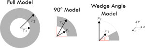
Before we move onto new material, let’s recap the problem. Here we were considering heat transfer through a cylinder with fixed inner and outer radial surface temperatures as in Figure 1. Given the geometry and boundary conditions, we could exploit the symmetry in this problem.

Cylindrical heat conduction with temperature boundary conditions — Figure 1 – The pipe under consideration for cylindrical heat transfer in OpenFOAM. The inner and outer radial surfaces are maintained at constant temperatures so heat can only flow in the radial direction.

Validation

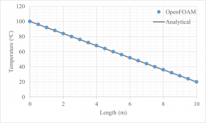
In the previous post we used OpenFOAM to compute the solution and Paraview to generate graphical and numerical data. We now want to validate this data against the exact analytical solution since there is one available for this case. The logarithmic equation that represents temperature as a function of radial location is shown in Eq. 1. Notice that thermal conductivity (or diffusivity) is not present here – as stated in the previous post this value is not important for this specific analysis. Hence it can be set to anything in OpenFOAM. Eq. 1 can easily be plotted in Excel alongside with the numerical data obtained from Paraview.

This plot has been done in Figure 2. The agreement between the two is excellent which suggests our OpenFOAM simulation, and post-processing steps with Paraview, work as intended. While this is great, we could even skip the use of Paraview and post-process the results mostly in OpenFOAM. “How?” you may ask, keep reading to find out.

T=\frac{T_1-T_2}{\ln(r_1/r_2)}\ln\left(\frac{r}{r_1}\right)+T_1\tag*{Eq. 1}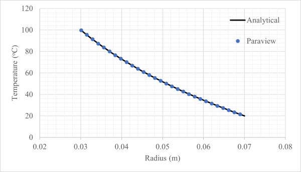

OpenFOAM cylindrical temperature distribution validation against analytical — Figure 2 – The validation of OpenFOAM results (with Paraview to post-process) against the exact analytical solution.

Post-processing with OpenFOAM

OpenFOAM comes with some post-processing capabilities out of the box which you can use for many simple tasks¹. While OpenFOAM cannot produce graphical results, it can produce the numerical data required by Excel to produce graphical results. Since most of us are more familiar with Excel than Paraview it is sometimes easier to stick with what we know. Still, Paraview is a great open-source tool so don’t forget about it²!

To do this in OpenFOAM, we need to use the postProcess command³. OpenFOAM needs to know the specific post-processing operations and what we are trying to find. For this we can use a dictionary file called sampleDict which is placed in the system folder of your case. Like most things in OpenFOAM, we’ll start with the basics before learning the more advanced concepts. A snippet of this file is shown below:


type		sets;
libs		(sampling);
fields		(T);

interpolationScheme	cellPoint;
setFormat		    raw;

sets
(
    line1
    {
        type    midPointAndFace;
        axis    xyz;
        start   (0.0 0.0 0.005);
        end     (0.1 0.1 0.005);
    }
);

Since we want to find the temperatures along a line, we need to set the type to sets and the fields to T. The libs entry just tells OpenFOAM where to look for some functionality but can actually be omitted from this example. The next two entries are a bit more interesting for us and we’ll go through each in a bit more detail.

interpolationScheme tells OpenFOAM how to interpolate values along the line. The line we define may not pass exactly through cell centroids, and if this is the case then we need to specify how to interpolate between the values. This can have an impact on the resulting values⁴. Here we will use cellPoint, but cellPointFace will also give reasonable results (the OpenFOAM website provides a description of these differences). You do not want to use cell here as this will not interpolate and instead just take the value at the cell centre for any data points which lay within the cell. This can result in a jagged line.
setFormat tells OpenFOAM the format to save the data in. There are a few useful options here – raw will write the data to a text file and csv will write the data to a comma separated value file. Either of these are fine for Excel but we have chosen raw.

After this we need to provide more information about the line(s) we want to sample data over. This is all contained within the sets subdictionary. We just need one entry since we are sampling data over a single line. Here we named the set line1 but it can be named anything. We then need to define a few entries for each set we have. We’ll go through some important entries for these below.

type refers to the sampling type and has many possibilities. We selected midPointAndFace but the options face and midPoint also give good results. These three options work slightly different to each other, but all will scale with the mesh resolution. Hence a larger number of mesh elements will result in more data points for these options. An alternative is uniform which just breaks the line into nPoints (this must be specified as well!) number of points and samples along these regardless of the mesh. More details of these can be found here.
axis tells how the location data is output. Here we have xyz which will give all coordinate data for each sample point to help plot the graph.
The start and end values are the x, y and z locations of the start and end of the line we wish to sample over. The points here were defined to work nicely with the case setup in the previous post but you can change this as required.

That’s all we need for sampleDict. Make sure this file is located in the system directory and then open your terminal and enter the command postProcess -func sampleDict.

Had you decided to change the name of your dictionary to something other than sampleDict, then replace that in the line above. If everything has been done correctly, then you should see a fair bit of text flash across the screen followed by End.

Now we need to look at the data produced by this sampling. Navigate to your case directory – you will see a folder called postProcessing has been created. Inside this you will find another folder named sampleDict (or the name of your dictionary file). Within this you will find more folders for each time step. Finally, within these folders you will find the result of the postprocess function for each set. If you used the raw format, then the files might have a .xy extension. This can be opened by any text viewer like Notepad++ or even just plain old Notepad. Once opened (as below), you can copy the data into Excel.


0.0212132 	0.0212132 	0.005 	100
0.0219203 	0.0219203 	0.005 	96.9369
0.0226274 	0.0226274 	0.005 	93.8738
...
0.0480833 	0.0480833 	0.005 	22.7295
0.0487904 	0.0487904 	0.005 	21.3647
0.0494975 	0.0494975 	0.005 	20

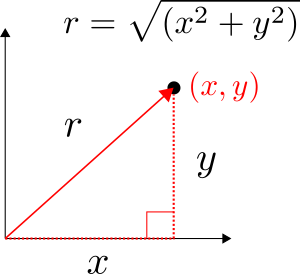
In this file, the columns correspond to the x, y, z coordinates and temperature, respectively. Notice that you have Cartesian coordinates but not a radial coordinate like used in Eq. 1. Never fear, you just need to perform some manipulation to get a radial coordinate from the x and y data. Once this is done you can plot the temperature distribution as a function of the radial location exactly like Eq. 1. You can do this by creating a new column in Excel for r and setting this equal to $\sqrt{x^2+y^2}$ . This can be done as the x and y point form a right-angle triangle which Pythagoras’ theorem applies to as shown in Figure 3.

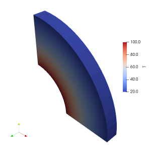
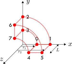
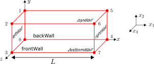
Notice in the output file we have 21 data points. This is not coincidental. Have a look at Figure 4 and the line which cuts through the mesh. There are 10 elements in the direction of the mesh. If you count all the cell midpoints and faces which intersect the line – the red dots in the left image – then you will get 21. Therefore we have 21 data points.

Converting Cartesian coordinates to radial coordinate — Figure 3 – The conversion of Cartesian (x and y) into radial (r) coordinates is simple using Pythagoras’ Theorem

OpenFOAM sampling types and mesh relation — Figure 4 – The number of data points in the output file is linked to the mesh and the sampling type. From left to right we have 21, 10 and 11 red dots.

If you count just the midpoints – the red dots in the middle image – then you will get 10. And if you count just the faces – the red dots in the right image – then you will get 11. Try changing the sampling type in sampleDict and see what happens to the number of data points. Now in Excel, you should be able to overlay the results onto the analytical temperature distribution from Eq. 1. Doing so produces Figure 5.

OpenFOAM post-process cylindrical temperature distribution validation against analytical — Figure 5 – The results of the OpenFOAM post-processing steps compared with the exact analytical solution. Paraview results in Figure 2 also agree with both.

Again, we have excellent agreement with the analytical solution. If you zoom in closely to the analytical curve, you will see there are slight discrepancies between the two values – the order of 0.1^oC. This is nothing to worry about for this analysis but it arises because we always have an approximate solution when using numerical methods. If you increase the mesh density (more mesh elements) then you will get closer to the analytical value. But you will also increase computational time so you need to balance these things out. For now, this mesh resolution is sufficient and we can consider this case validated.

This completes the basic use of post processing in OpenFOAM using dictionary files. Once you have setup these files, you will find yourself using them for many cases and just making adaptations on the fly. The postProcess command in OpenFOAM is faster than any graphical user interface and is particularly well suited for programmatic approaches, large simulations and repeated simulations. Obviously more complex tasks can be performed, but what we have done here is a good entry point.

Summary

In the previous few posts we have validated a case of radial heat conduction in a pipe using OpenFOAM. Along we way we learnt how to use blockMesh to create cylinders and had some exposure to post-processing in Paraview and with OpenFOAM. The results of our numerical simulation agreed very well with theoretical predictions. The case files for these simulations can be downloaded via this link.

In the next post, we are going to refine the model and geometry we came up with in the previous few posts which will introduce some new methods and techniques to our toolkit.