Cylindrical Heat Conduction Equation with Convective Boundary

In the previous post we looked at the solution to the steady, one-dimensional cylindrical heat equation with flux boundary conditions. In this post we will look at another solution to this conduction equation, but now with convective boundary conditions. This is probably the most useful equation for the cylindrical system since these equations are often useful for pipe flow scenarios which is very common in engineering. This analysis can help us to find the temperature distribution and thus the rate of heat loss or gain from a pipe.

Convective boundary conditions for radial heat conduction equation — Figure 1. The steady radial system with convective boundary conditions.

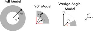
For the steady, one-dimensional system considered in Figure 1, the general solution to the heat equation is presented in Eq. 1. Note that this is sometimes called a radial system as heat only flows in the radial ( $r$ ) direction. Such a system exists within pipes of circular cross-sections where radial heat flow corresponds to heat passing through the pipe wall. We can take the derivative of Eq. 1 to find the temperature gradient within the system, as shown in Eq. 2. This helps us formulate the system of equations to solve to find the constants $A$ and $B$ .

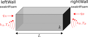
T=A\ln(r)+B \tag*{Eq. 1}

\frac{dT}{dr}=\frac{A}{r} \tag*{Eq. 2}

The convective boundary conditions on the inner and outer surface are shown in Figure 1. Convection on the inner surface occurs via a fluid with mean temperature $T_A$ and heat transfer coefficient $h_A$ . On the outer surface, convection occurs via a fluid with free-stream temperature of $T_B$ and heat transfer coefficient $h_B$ . The thermal conductivity is fixed at $k$ for the solid region. The boundary conditions are shown for the left and right boundary in BC 1 and BC 2, respectively. At this point, we should be familiar with the process for formulating the boundary conditions as this has been done in previous posts.

h_A(T_A-T_i)=\left.-k\frac{dT}{dr}\right|_{r_i} \tag*{BC 1}

h_B(T_o-T_B)=\left.-k\frac{dT}{dr}\right|_{r_o} \tag*{BC 2}

Working with these expressions to arrive at a unique solution that depends only on fluid temperatures $T_A$ and $T_B$ is a little bit tricky. To start, we can evaluate expressions for $T_i$ and $T_o$ using Eq. 1. Here we will get $T_i=A\ln(r_i)+B$ and $T_o=A\ln(r_o)+B$ . These can be substituted into BC 1 and BC 2, along with Eq. 2 as required. After doing this, we end up with the expressions shown in Eq. 3 and Eq. 4.

h_A(T_A-(A\ln(r_i)+B))=-k\frac{A}{r_i} \tag*{Eq. 3}

h_B((A\ln(r_o)+B)-T_B))=-k\frac{A}{r_o} \tag*{Eq. 4}

Dividing both of these by the leading convective term makes the equations easier to solve.

T_A-(A\ln(r_i)+B)=-\frac{k}{h_Ar_i}A \tag*{Eq. 5}

(A\ln(r_o)+B)-T_B=-\frac{k}{h_Br_o}A \tag*{Eq. 6}

We start to see a familiar grouping appear. The Biot number is defined as $Bi=hL/k$ and the inverse of this is present on the right hand side of both equations (note that $L$ is just a characteristic length which can be taken as the radius in this case). This dimensionless quantity is very important in heat transfer as it relates the magnitude of resistances associated with convection and conduction. This will be covered more in future posts. We now need to solve Eq. 5 and Eq. 6 for $A$ and $B$ . We can add these equations together as this will eliminate $B$ and leave an expression in terms of $A$ .

\begin{align*} T_A-A\ln(r_i)-B&=-\frac{k}{h_Ar_i}A \\ +\biggr( A\ln(r_o)+B-T_B &=-\frac{k}{h_Br_o}A \biggr) \\ A\ln(r_o)-A\ln(r_i)+T_A-T_B &=-\frac{k}{h_Ar_i}A-\frac{k}{h_Br_o}A \end{align*}

After simplifying this expression we get the following for $A$ .

A=\frac{T_B-T_A}{\ln(\frac{r_o}{r_i})+\frac{k}{h_Ar_i}+\frac{k}{h_Br_o}} \tag*{Eq. 7}

We can then find $B$ by rearranging either Eq. 5 or Eq. 6 in terms of $B$ and substituting in the value for $A$ in Eq. 7. If we were to rearrange Eq. 5, then we would obtain the following for $B$ .

B=T_A-\left(\ln(r_i)-\frac{k}{h_Ar_i} \right)A

B=T_A-\left(\ln(r_i)-\frac{k}{h_Ar_i} \right)\left( \frac{T_B-T_A}{\ln(\frac{r_o}{r_i})+\frac{k}{h_Ar_i}+\frac{k}{h_Br_o}} \right) \tag*{Eq. 8}

Note that we could have alternatively rearranged Eq. 6 in terms $B$ and obtained a slightly different expression for $B$ with $T_B$ and $r_o$ . Either way will work. Now we can substitute both $A$ and $B$ into the general solution of Eq. 1. After some simplifications we end up with Eq. 9.

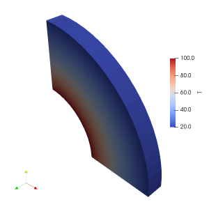
T=T_A+ \frac{T_B-T_A}{\ln(\frac{r_o}{r_i})+\frac{k}{h_Ar_i}+\frac{k}{h_Br_o}} \left[ \ln\left(\frac{r}{r_i} \right)+\frac{k}{h_Ar_i}\right] \tag*{Eq. 9}

This is the temperature distribution within a steady, radial system with convective boundary conditions on the inner and outer wall. With it we can find the rate of heat transfer through circular pipes with fluid flowing inside and around them. This pipe flow scenario is widely applicable in real life and so this equation is very useful. In the next post, we will summarise some of the more important concepts that we have covered in the previous series of posts.