Cylindrical Heat Conduction Equation with Flux Boundaries

Over the last few posts we have looked at solutions to the one-dimensional, steady Cartesian heat equation. In this post we will go over the process of finding solutions for the cylindrical heat equation. More specifically, we will consider one-dimensional, steady heat flow which ends up being the radial heat equation. The process here is quite similar to the Cartesian system since in both cases we have an ordinary differential equation with two boundary conditions. We have a different starting ODE for the radial case and as such get a slightly different solution. The general solution and derivative for the steady radial system can be expressed in Eq. 1 and Eq. 2, respectively. This was covered here.

T=A\ln(r)+B \tag*{Eq. 1}

\frac{dT}{dr}=\frac{A}{r} \tag*{Eq. 2}

We need to use the boundary conditions to find the values for $A$ and $B$ . We will look at flux boundary conditions and some of the interesting results produced by these.

Two flux boundary conditions

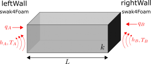
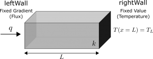
We can consider the case shown in Figure 1 which is a radial system with flux boundary conditions on both the inside and outside radial surface. Here we have flux $q_i$ entering through the boundary at $r_i$ and flux $q_o$ leaving through the boundary at $r_o$ . The thermal conductivity of the solid is $k$ .

If we remember back to the equivalent Cartesian system with two flux boundary conditions, there was no unique solution for this case. The best we could come up with was a family of solutions. The same thing happens with the radial system – we cannot find a unique solution. However we do come up with a useful relation through this analysis so we’ll proceed anyway. The boundary conditions for the left and right wall are shown in BC 1 and BC 2.

q_i=-k\left. \frac{dT}{dr}\right|_{r_i} \tag*{BC 1}

q_o=-k\left. \frac{dT}{dr}\right|_{r_o} \tag*{BC 2}

We can substitute Eq. 2 into BC 1 and BC 2. We need to remember to replace $r$ with $r_i$ and $r_o$ as required in Eq. 2. The following can be obtained for $A$ .

q_i=-k\frac{A}{r_i}

A=-\frac{q_ir_i}{k}

q_o=-k\frac{A}{r_2}

A=-\frac{q_or_o}{k}

We know that $A$ is a constant and $k$ is the thermal conductivity which is also a constant. Using this, we can come up with the following relation for the radial system.

q_ir_i=q_or_o \tag*{Eq. 3}

Eq. 3 is very useful and tells us that the flux multiplied by the radius at the inside wall must be equal to the flux multiplied by the radius at the outside wall. This can actually be generalised to any radial location within the system and hence this value must be conserved throughout the system. It’s important to note that within the Cartesian system the flux itself i.e. $q$ was the value that was constant. However here we must keep constant the flux multiplied by the radius at that location. This distinction is due to the fact that as the radius increases, so too will the circumference of the circle at that radius. With this in mind, we can recognise that this useful expression really stems from conservation of energy principles within the system.

There is no point trying to come up with a solution to the system in Figure 1. It can’t be done as there is no more information contained within BC 1 and BC 2 and so we have no ability to find the constant $B$ .

Flux and Temperature

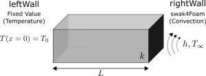
If we were to fix the inside temperature to a value $T_i$ and keep the outer surface a flux boundary then we would have the system as shown in Figure 2. In this case it would be possible to find the temperature distribution.

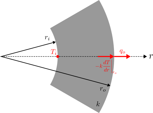
Temperature and flux boundary conditions for radial heat conduction equation — Figure 2. The steady radial system with temperature and flux boundary conditions.

The boundary conditions are listed in BC 3 and BC 4.

T(r_i)=T_i \tag*{BC 3}

q_o=-k\left. \frac{dT}{dr}\right|_{r_o} \tag*{BC 4}

The constant $A$ is still equal to $-q_or_o/k$ as above so we just need to find the constant $B$ . Here we can use BC 3 and substitute this into the general solution which has been done below.

T=A\ln(r)+B

T_i=A\ln(r_i)+B

T_i=-\frac{q_or_o}{k}\ln(r_i)+B

B=T_i+\frac{q_or_o}{k}\ln(r_i)

We can then substitute both $A$ and $B$ into the general solution and simplify using log laws to obtain the temperature distribution in Eq. 4.

T=T_i+\frac{q_or_o}{k}\ln\left(\frac{r_i}{r}\right) \tag*{Eq. 4}

If we were to swap the temperature and flux boundary conditions in Figure 2 (temperature on the right and flux on the left), then we would arrive at a slightly different result for the temperature distribution as shown in Eq. 5.

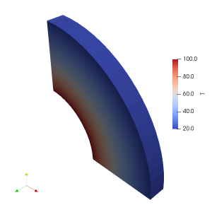
T=T_o+\frac{q_ir_i}{k}\ln\left(\frac{r_o}{r}\right) \tag*{Eq. 5}

In either case, both of these equations allow us to plot the temperature distribution within a radial system with one heat flux boundary and one temperature boundary. This can be useful for finding the temperature within pipe walls. In the next post, we are going to look at solving the same radial heat equation, but with convective boundary conditions.