How to Analytically Solve the Cartesian Heat Equation

We have now had a brief introduction to solving the heat conduction equation through analytical methods in a previous post. In this post, we will provide the full analytical solution, starting with the simplest of cases: the steady state, one-dimensional Cartesian system. We are also going to start looking at the importance of boundary conditions and how they can influence the solution.

Steady, One-Dimensional Cartesian Heat Equation

The 3D heat equation in Cartesian coordinates can be expressed in Eq. 1 (we derived this here). Considering steady, one-dimensional heat transfer eliminates the time derivative (since it is steady state) and two of three spatial derivatives (since it is one-dimensional). It doesn’t really matter which spatial derivatives are eliminated (the solution will be the same either way), but it is convention to leave the $x$ direction. After doing this, we arrive at Eq. 2. This is an ordinary differential equation (ODE) which is far easier to solve than the partial differential equation in Eq. 1. For an ODE the $\partial$ is replaced with $d$ for the differential term.

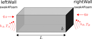
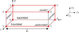
\frac {\partial^2T}{\partial x^2}+\frac {\partial^2T}{\partial y^2}+\frac {\partial^2T}{\partial z^2} =\frac{1}{\alpha} \frac {\partial T}{\partial t} \tag*{Eq. 1}

\frac {d^2T}{d x^2} =0 \tag*{Eq. 2}

It might be a good idea to appreciate what such a system might look like. This is a system where heat can only transfer in one direction. Some examples of these are walls, slabs and insulated bars as shown in Figure 1.

Cartesian one dimensional heat transfer — Figure 1. Some examples of one-dimensional Cartesian heat transfer systems.

Solving this ODE is quite simple and only requires integration twice to arrive at the general solution. This process has been shown below.

\int\frac {d^2T}{d x^2}dx =\int 0 dx

\frac {dT}{d x}=A\tag*{Eq. 3}

\int\frac {dT}{d x} dx=\int A dx

T= Ax+B\tag*{Eq. 4}

Thus the general solution is $T= Ax+B$ . Since $A$ and $B$ are constants the solution must be a straight line.

It’s useful again to think about the above process. Eq. 2 states that the second derivative of temperature with respect to the $x$ direction must be zero. The second derivative relates to curvature and this implies there is no curvature in the function $T(x)$ since its second derivative is zero. A function that has zero curvature everywhere is a straight line. Think of other functions – $y=x^2$ , $y=x^{1/3}$ , $y=e^x$ and $y=\sin x$ – all of these have some curvature in them and thus cannot be a solution to this ODE.

Similarly, think about Eq. 3 which states that the first derivative of temperature with respect to the $x$ direction must be a constant ( $A$ ). The first derivative relates to a functions gradient and the only function which has a constant gradient is again a straight line. Functions like $y=x^2$ , $y=x^{1/3}$ , $y=e^x$ and $y=\sin x$ have varying gradients thus cannot be a solution to this ODE.

We don’t yet know what $A$ and $B$ are and need to use the boundary conditions to find these constants. Since our original ODE had second derivatives, there needs to be two boundary conditions to completely solve the problem. These represent the conditions at each boundary of the problem and they are needed to “lock” the solution in space. This is because there are lots of possible straight lines that satisfy the ODE – remember that $A$ and $B$ can be any constant.

To help visualise this, look at Figure 2. Each of these straight lines will satisfy the ODE since there second derivative is equal to zero, but they all can’t be solutions to our particular problem. Although we know the solution must be a straight line, we aren’t sure exactly where the line begins or ends. This is what the boundary conditions will help us figure out.

Cartesian one dimensional heat transfer possible solutions — Figure 2. There are many possible straight lines which satisfy the heat equation. The boundary conditions help us figure out the right one.

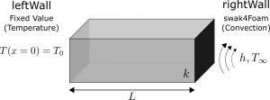
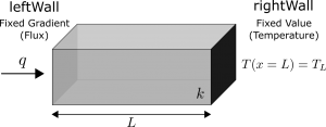
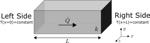
The simplest boundary conditions to consider are fixed temperature boundary conditions. These can be mathematically formulated in BC 1 and BC 2. BC 1 states that the temperature at $x=0$ is equal to $T_1$ and BC 2 states that the temperature at $x=L$ is equal to $T_2$ . This is like fixing the temperature on the left and right boundaries of the wall in Figure 2.

T(x=0)= T_1 \tag*{BC 1}

T(x=L)= T_2 \tag*{BC 2}

These two boundary conditions can be substituted into Eq. 4 to solve for $A$ and $B$ . This simple process leads to values for $A$ and $B$ as in Eq. 5 and Eq. 6, respectively. Note that $L$ is the length as shown in Figure 2.

A=\frac{T_2-T_1}{L} \tag*{Eq. 5}

B=T_1 \tag*{Eq. 6}

These can now be substituted into Eq. 4 to arrive at the particular solution:

T=\left(\frac{T_2-T_1}{L}\right)x+T_1 \tag*{Eq. 7}

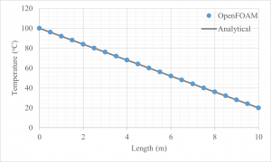
Cartesian one dimensional heat transfer solution — Figure 3. The temperature distribution in a Cartesian system.

Eq. 7 is the particular solution for one dimensional, steady heat transfer through a rectangular system with fixed end temperatures. With it the temperature distribution can be plotted as shown in Figure 3 to the side.

We can now figure out the temperature distributions in many common objects. Another common object engineers deal with are pipes and unfortunately this equation cannot predict the temperature distribution within a pipe wall. For that, we need to solve the cylindrical heat equation, which we will do next time.