How to Analytically Solve the Spherical Heat Equation

In two previous posts we looked at the analytical solution to simplified Cartesian and cylindrical heat conduction equations. These two systems actually cover a lot of practical scenarios we might want to consider. Another situation that arises, although less common than the previous two, is a spherical system. Pressure vessels occasionally are designed with spherical shapes so it is possible we would want to know the temperature distribution through the shell. In this case, we need to solve the steady, one-dimensional spherical heat equation which is the simplest form of the spherical heat equation.

Steady, One-Dimensional Spherical Heat Equation

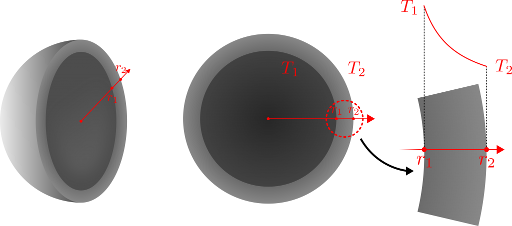
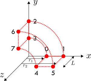
The spherical heat equation has been shown in Eq. 1 for a constant thermal conductivity solid. Since we are interested in the steady solution, the time derivative will be zero and we are left with three spatial derivatives. Practically, the situation with radial ( $r$ ) heat transfer as shown in Figure 1 is most common. In this system, radial temperature variations are present throughout the shell, but no temperature variations in either the azimuth ( $\phi$ ) or polar ( $\theta$ ) directions are present. These simplifications lead to an ordinary differential equation (ODE) as shown in Eq. 2.

\frac{1}{r^2}\frac {\partial}{\partial r}\left(r^2\frac{\partial T}{\partial r}\right)+\frac{1}{r^2\sin^2\theta}\frac {\partial^2T}{\partial^2 \phi}+\frac{1}{r^2\sin\theta}\frac {\partial}{\partial \theta}\left(\sin\theta\frac{\partial T}{\partial \theta}\right) = \frac{1}{\alpha}\frac {\partial T}{\partial t} \tag*{Eq. 1}

\frac{1}{r^2}\frac {d}{d r}\left(r^2\frac{d T}{d r}\right) = 0

\frac {d}{d r}\left(r^2\frac{d T}{d r}\right) = 0 \tag*{Eq. 2}

Note that we can neglect the $1/r^2$ term since this can’t be equal to zero and thus are only left with the derivative. We can integrate Eq. 2 twice to obtain the general solution to the ODE.

\int\frac {d}{d r}\left(r^2\frac{d T}{d r}\right)dr = \int0dr

r^2\frac{d T}{d r} = A

\frac{d T}{d r} = \frac{A}{r^2}

\int\frac{d T}{d r}dr = \int\frac{A}{r^2}dr

T = -\frac{A}{r}+B \tag*{Eq. 3}

The general solution is shown in Eq. 3 and is a hyperbola of the form $T = -A/r+B$ . This is unlike the straight line solution for the Cartesian system and the logarithmic solution for the cylindrical system.

The boundary conditions are now required to find the constants $A$ and $B$ . The simplest boundary conditions are the fixed temperature conditions as shown in BC 1 and BC 2. These conditions hold the temperature on each side of the shell at a fixed value. BC 1 states that the temperature at $r=r_1$ is equal to $T_1$ and BC 2 states that the temperature at $r=r_2$ is equal to $T_2$ .

T(r=r_1) = T_1\tag*{BC 1}

T(r=r_2) = T_2\tag*{BC 2}

These can be substituted into the general solution of Eq. 3 and solved simultaneously. This yields values for $A$ and $B$ as in Eq. 4 and Eq. 5. The particular solution is represented in Eq. 6.

A = \frac{r_1r_2}{r_1-r_2}(T_1-T_2)\tag*{Eq. 4}

B = \frac{r_1T_1-r_2T_2}{r_1-r_2}\tag*{Eq. 5}

T = -\frac{r_1r_2}{r(r_1-r_2)}(T_1-T_2)+\frac{r_1T_1-r_2T_2}{r_1-r_2}\tag*{Eq. 6}

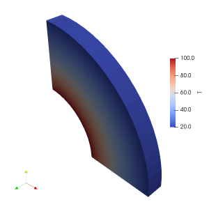
Spherical one dimensional heat transfer — Figure 1. The system under consideration.

We can now plot the temperature distribution within a spherical shell. This has been shown in Figure 1. This completes the analytical solutions for the steady, one-dimensional heat equations in each coordinate system.

Throughout these derivations we have assumed the simplest boundary condition – fixed temperature at the boundary. Although this is very useful, it’s not always practical. In the next few posts we will look at different boundary conditions and how they influence analysis of the heat equation.