We have spent many posts discussing the origins of the heat conduction equation, it naturally follows we would want to try to solve this. Once solved, we will know the temperature everywhere within the solid at all times. This is the ultimate goal of all of this. Unfortunately, solutions are not easy to obtain. This is because the heat equation is a partial differential equation (PDE) – these generally are difficult to solve. The literature on solving PDEs is far too extensive to cover in a few posts (think more of a textbook!). So here we are briefly going to cover some ways we can solve the heat equation with a focus on analytical methods in this post.
Analytical
We used analytical methods to derive the heat equation in various coordinate systems. We obtained PDEs so the most logical way of solving these is by continuing with the analytical methods that got us here in the first place. An analytical solution is one that looks like:
T=f(x,y,z,t)
This gives us the temperature within the solid as a function of spatial coordinates and time. The key here is to find a mathematical expression for f that satisfies the original PDE (and boundary/initial conditions – more on these later). If we could find the functional form of f , then we’d be very happy! However we can only find this for a small number of cases. These cases all rely on first applying simplifications to the heat equation thus making it a simpler PDE to solve. In some cases even an ordinary differential equation (ODE) results. These solutions are still practical and there is much we can learn from them.
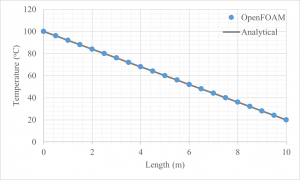
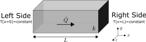
Perhaps the most simple analytical solution to the heat equation is for the steady-state, one-dimensional Cartesian system. We can imagine this as a solid wall with each side held at a different temperature. The solution in this case has the form T=f(x) since it is steady and one-dimensional and the form of f can be easily found by solving the ODE. The solution happens to be a straight line i.e. T=Ax+B . We still need to find A and B , which relate to the boundary conditions, but will leave that for another time. This means that temperature varies linearly throughout the wall as shown below.

A slightly more complicated analytical solution is for the steady-state, one-dimensional cylindrical system. We can imagine this as a pipe with inside and outside walls held at different temperatures. The solution is of the form T=f(r) since it is steady and one-dimensional. We are solving a different ODE in this case for the cylindrical system. The solution is not a straight line – it has the form T=A\ln r + B . Again, we need to find A and B but neglect them for now. For this system, temperature varies logarithmically as below. This is more complex than the linear manner for the Cartesian system but still rather simple.

We can even do this for a spherical object. Using the ODE produced by the one-dimensional, steady spherical heat equation we can imagine a hollow sphere with each side held at different temperatures. The solution here is not a straight line nor a logarithmic line, instead we end up with something of the form T=-A/r + B . Again, we can ignore A and B for now. The temperature varies inversely with the radius in this spherical system.
The mathematics involved in these three solutions is actually fairly simple since we considered a steady and one-dimensional system. This reduced the PDE to an ODE and thus the dependent variable ( T ) only varied with one independent variable ( x or r ).
As soon as we consider a PDE, the dependent variable ( T ) can depend on multiple independent variables, for example x and t or r and t , and our solution becomes much harder to find. The mathematics involved can quickly become unwieldy and the solutions become more difficult to use as well. For the unsteady, one-dimensional Cartesian system, the general solution is of the form:
T(x,t)=\sum_{n=1}^\infty b_n\sin\left(\frac{n \pi}{L}x \right) \exp\left[{-\left(\frac{n\pi}{L}\right)^2 \alpha t}\right]This is significantly more complicated than the solution for the steady, one-dimensional Cartesian system which was a straight line. We can also find the solution for the steady, two-dimensional Cartesian system. For a particular case of this, its solution is of the form:
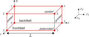
\theta(x,y)=\frac{2}{\pi}\sum_{n=1}^\infty \frac{(-1)^{n+1}+1}{n}\sin\left( \frac{n\pi x}{L}\frac{\sinh(n\pi y/L)}{\sinh(n\pi W/L)} \right)Here \theta (x,y) is a non-dimensional temperature. Again we find that the solution is quite complex.
Both of these solutions require infinite series. This means that to find the temperature at a particular point for any of these two cases, we need to sum an infinite series. Then and only then will we get the exact solution. The two-dimensional, steady-state solution also requires hyperbolic functions. When we look deeper into the one-dimensional, transient solution we will find a need for Fourier series as well. Practically, solving these becomes a bit of a problem due to these complexities.
What we can conclude from this is that even though we can find an analytical solution for some cases, it doesn’t necessarily mean that we should find it. It may or may not be the best option for us and we need to use some discretion here. For even more complicated problems than the ones mentioned here, analytical solutions can become so complex that they are hardly worth using. For these cases, and for the cases where analytical solutions are not mathematically possible, we might want to look at numerical solutions which is what we will cover in the next post.
Read more from Qdot Systems…
A Better Way to Make Cylinders in OpenFOAM
In the previous posts we looked at creating cylinders in OpenFOAM and running heat conduction…
A Look at Cylindrical Heat Transfer in OpenFOAM: Part 3
We’ll continue exploring cylindrical heat transfer in OpenFOAM in this post. At the end of…
A Look at Cylindrical Heat Transfer in OpenFOAM: Part 2
A Look at Cylindrical Heat Transfer in OpenFOAM: Part 1
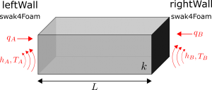
How To Combine Thermal Boundary Conditions in OpenFOAM
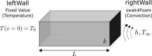
Convective Boundary Condition for the 1D Heat Equation in OpenFOAM
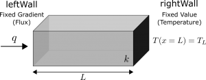
Flux Boundary Condition for 1D Heat Equation in OpenFOAM
How to Solve the Heat Conduction Equation with OpenFOAM (3)
How to Solve the Heat Conduction Equation with OpenFOAM (2)
How To Solve The Heat Conduction Equation With OpenFOAM (1)
A Brief Introduction to CFD Using OpenFOAM
